Calculate Global Minimum Variance Portfolio Using R

In this and the next couple of posts, I’ll give examples of how to calculate optimized portfolios using R and the vanguard funds in my retirement account. Today, I’ll show you how to calculate the global minimum variance portfolio, which was the first major result in Markowitz’s portfolio theory. Given a collection of assets, their global minimum variance portfolio is the portfolio with the smallest portfolio volitility.

Step 0. Load libraries and define helper functions

library(zoo)
library(tseries)

download_data = function(symb, begin, end) {
        get.hist.quote(instrument=symb, start=begin, end=end, 
                       origin="1970-01-01", quote="AdjClose", 
                       provider="yahoo", compression="m", 
                       retclass="zoo")
}

to_yearmon = function(data) {
        index(data) = as.yearmon(index(data))
}

Step 1. I choose assets from three broad classes: stocks, bonds, and commodities. For stocks, I choose funds that cover total US market, total international markets, and real estate. For bonds, I choose funds that invest in the total US bond market and inflation protected securities. For commodities, I choose funds that invest in gold and other precious metals and their mining companies and oil & gas and energy companies. First, I download the monthly adjusted closing price data of these funds between June 2000 and Oct 2014 from Yahoo.

# initialize the fund symbols 
stocks = c("VTSMX", "VGTSX", "VGSIX")
bonds = c("VIPSX", "VBMFX")
commodities = c("VGPMX", "VGENX")
symbols = c(stocks, bonds, commodities)

# download adj. price data
port = list()
for (symbol in symbols)
        port[[symbol]] = download_data(symbol, "2000-06-29", "2014-10-31")

# change the class of the time index to yearmon
lapply(port, to_yearmon)

# put both all price data in one data frame
prices = do.call("cbind", port)
colnames(prices) = symbols

Step 2. Calculate monthly continuously compounded returns as difference in log prices.

ret.cc = diff(log(prices))

# inspect the return data
cat("Start: ", as.character(start(ret.cc)), "  End: ", as.character(end(ret.cc)))

## Start:  2000-07-03   End:  2014-10-01

head(ret.cc, 3)

##                  VTSMX        VGTSX       VGSIX        VIPSX       VBMFX
## 2000-07-03 -0.01971716 -0.045649607  0.08408300  0.007936630 0.008832746
## 2000-08-01  0.07027806  0.009904851 -0.04071584  0.006893088 0.013956404
## 2000-09-01 -0.04782406 -0.051333260  0.02899155 -0.004918734 0.007621014
##                  VGPMX       VGENX
## 2000-07-03 -0.01628457 -0.04730217
## 2000-08-01  0.11545891  0.11519991
## 2000-09-01 -0.07451730  0.01346586

Step 3. Calculate the sample average returns of the underlying assets and the sample covariance matrix of the returns.

mu.hat.annual = apply(ret.cc, 2, mean) * 12   
cov.mat.annual = cov(ret.cc) * 12

Step 4. Finally, we can calculate the global minimum variance portfolio using a helper function written by Eric Zivot and Hezky Varon from U of Washington.

helper = "~/Coding/R-related/R/portfolio-optim/portfolio_noshorts.r"
source(helper)
global.minvar.port = globalMin.portfolio(mu.hat.annual, cov.mat.annual, short=F)

global.minvar.port

## Call:
## globalMin.portfolio(er = mu.hat.annual, cov.mat = cov.mat.annual, 
##     shorts = F)
## 
## Portfolio expected return:     0.05214958 
## Portfolio standard deviation:  0.03355 
## Portfolio weights:
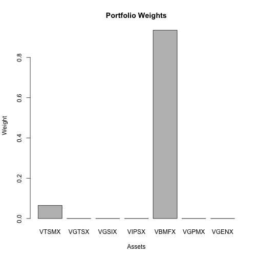
## VTSMX VGTSX VGSIX VIPSX VBMFX VGPMX VGENX 
## 0.065 0.000 0.000 0.000 0.935 0.000 0.000

# port weights
plot(global.minvar.port)

center

Categories