Analyze Stock Price Data Using R, Part3

When analyzing stock returns, we like to know if the average returns or volatilities are constant over time, or if the correlations between any two assets in our portfolio stay constant over time. Therefore, we need to pick a time windows and calculate the rolling means, volatilities or correlations. A common choice for a time window is 2 years. However, in practice, I often pick several time windows of different length (like 6 months, 1 year, 2 years, 5 years) and compare the results obtained under each time window. The function rollapply() in the zoo library allows us to calculate the rolling statistics easily.

Step 1. Load libraries

library(PerformanceAnalytics)
library(zoo)
library(tseries)

Step 2. Download the monthly adjusted closing price data on VGENX and VTSMX since Sept 2005 from Yahoo.

VGENX = get.hist.quote(instrument="VGENX", start="2005-09-30", 
                       end="2014-09-30", origin="1970-01-01",
                       quote="AdjClose", provider="yahoo", 
                       compression="m", retclass="zoo")

## time series ends   2014-09-02

VTSMX = get.hist.quote(instrument="VTSMX", start="2005-09-30", 
                       end="2014-09-30", origin="1970-01-01",
                       quote="AdjClose", provider="yahoo",
                       compression="m", retclass="zoo")

## time series ends   2014-09-02

Step 3. Change the class of the time index to yearmon.

index(VGENX) = as.yearmon(index(VGENX))
index(VTSMX) = as.yearmon(index(VTSMX))

Step 4. Merge both price series into one data frame and Calculate continuously compounded returns.

prices = merge(VGENX, VTSMX)
colnames(prices) = c("VGENX", "VTSMX")
ret.cc = diff(log(prices))
head(ret.cc, 3)

##                VGENX        VTSMX
## Oct 2005 -0.08818443 -0.018813600
## Nov 2005  0.02153350  0.038941761
## Dec 2005  0.03146979  0.001354186

Step 5. Calculate and Chart the rolling mean of the cc returns.

time.window = c(6, 12, 24, 60)

for (m in time.window) {
        roll.muhat = rollapply(ret.cc, width=m, FUN=mean, align="right")
        chart.TimeSeries(roll.muhat, legend.loc="bottomright", 
                         main = paste("rolling period:", m, "months"), 
                         ylab="rolling mean of the cc returns")
}

center center center center

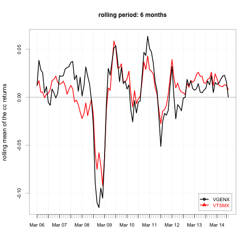
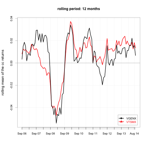
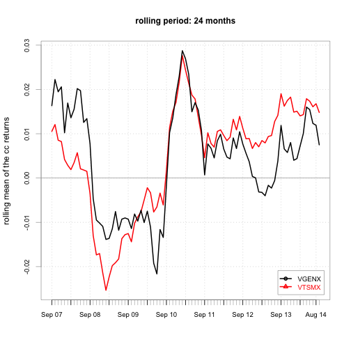
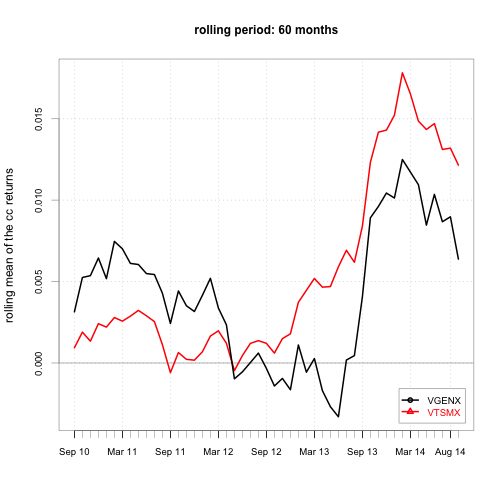
Note that neither security has a constant monthly cc return.

Step 6. Calculate and Chart the rolling mean of the volatilities.

for (m in time.window) {
        roll.sigmahat = rollapply(ret.cc, width=m, FUN=sd, align="right")
        chart.TimeSeries(roll.sigmahat, legend.loc="bottomright", 
                         main = paste("rolling period:", m, "months"), 
                         ylab="rolling volatility of the cc returns")
}

center center center center

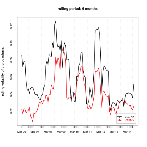
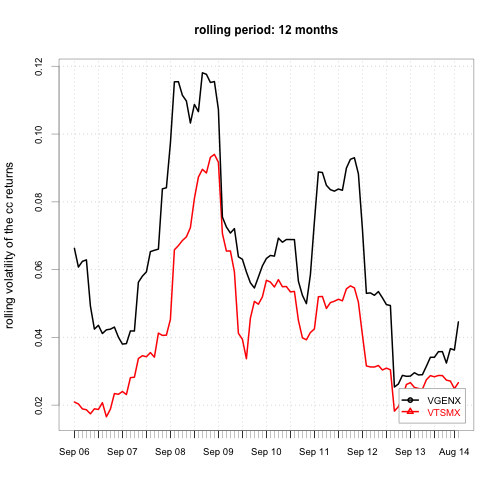
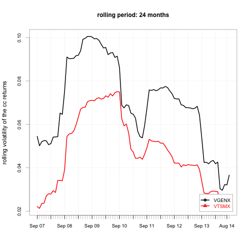
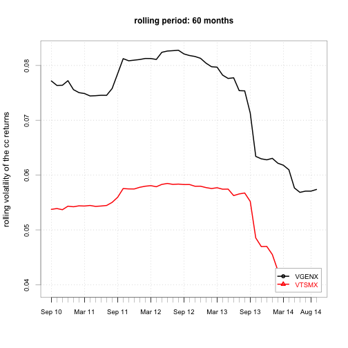
We see the volatilities of both securities are changing over time too.

Step 7. Calculate and Chart the rolling correlation between the two return series.

rhohat = function(x) cor(x)[1, 2]

for (m in time.window) {
        # set by.column=FALSE to apply FUN to both cols at once
        roll.rhohat = rollapply(ret.cc, width=m, FUN=rhohat, by.column=FALSE, 
                                align="right") 
        chart.TimeSeries(roll.rhohat,
                         main = paste("rolling period:", m, "months"), 
                         ylab="rolling correlation of the two cc return series")
}

center center center center

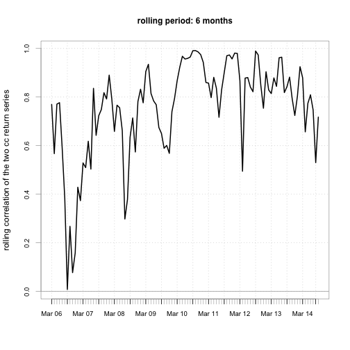
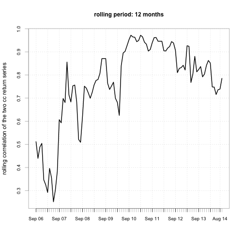
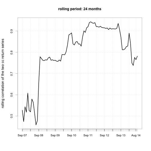
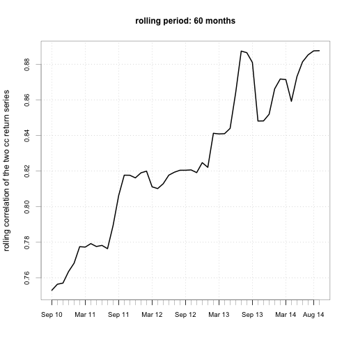
We see the correlations between the returns of VTSMX (all stocks) and VGENX (energy stocks) are NOT constant overtime. Between 2006 and 2007, their correlation is small, and sometimes is even close to zero, but during the financial crisis of 2007 - 2011, they are highly correlated. You’ll see this a lot in other pairs of securities. In general, assets are not correlated during normal time will become highly correlated during crisis. As my old finance professor liked to say, “Diversification helps except when the world is on fire. And some day, the world will be on fire.”

Categories