Analyze Stock Price Data Using R, Part1

Crude oil has been hammered. Yesterday, it hit the lowest price in 2 years. Being a contrarian, I smell the opportunity to buy. My interest is a vanguard energy fund (VGENX), which has 95% of its assets invested in oil or oil related sectors. Let’s first take a look at its prices and returns histories since Sept 2005.

Step 1. Load libraries and helper functions

library(PerformanceAnalytics)
library(zoo)
library(tseries)

plt_dist = function(dat, varname) {
        # Creates a figure of 4 plots: histogram, boxplot, 
        #                              density curve, qqplot
        #
        # Args:
        #       dat     : a data frame or matrix with colnames
        #       varname : a string specifying the numerical variable 
        #                 in dat to be drawn
        #
        # Returns:
        #       draws 4 plots (histogram, boxplot, density curve, 
        #       qqplot) on one canvas
        par(mfrow = c(2,2))
        hist(dat[, varname], main="histogram", xlab=varname, 
             probability=TRUE, col=hcl(h=195,l=65,c=100))
        boxplot(dat[,varname], outchar=TRUE, main="boxplot", cex=0.7, 
                xlab=varname, col=hcl(h=195,l=65,c=100))
        plot(density(dat[,varname]), type="l", 
             main="Smoothed density", lwd=2,
             xlab=varname, ylab="density estimate", 
             col=hcl(h=195,l=65,c=100))
        qqnorm(dat[,varname], col=hcl(h=195,l=65,c=100), cex=0.7)
        qqline(dat[,varname])
        par(mfrow=c(1,1))
}

Step 2. Download the monthly adjusted closing price data on VGENX since Sept 2005 from Yahoo!.

VGENX = get.hist.quote(instrument="VGENX", start="2005-09-30", 
                       end="2014-09-30", origin="1970-01-01",
                       quote="AdjClose", provider="yahoo", 
                       compression="m", retclass="zoo")

## time series ends   2014-09-02

Step 3. Change the class of the time index to yearmon.

index(VGENX) = as.yearmon(index(VGENX))
colnames(VGENX) = c("VGENX")

Step 4. Calculate continuously compounded returns.

ret.cc = diff(log(VGENX))
head(ret.cc, 3)

##                VGENX
## Oct 2005 -0.08818443
## Nov 2005  0.02153350
## Dec 2005  0.03146979

Step 5. Plot prices.

chart.TimeSeries(VGENX, legend.loc="bottomright", main="", 
                 ylab="monthly adj. closing prices")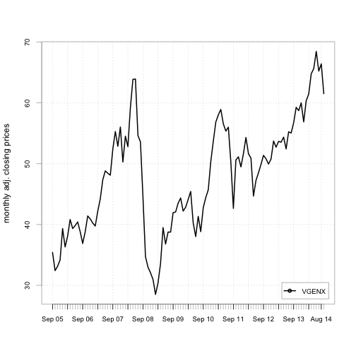

center

Step 6. Plot cumulative returns.

ret.simple = diff(VGENX) / lag(VGENX, k=-1)
chart.CumReturns(ret.simple, legend.loc="topleft", wealth.index=TRUE, 
                 ylab="$", main="Future Value of $1 invested")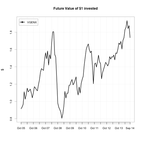

center

Step 7. Plot the distribution of cc returns.

# Create matrix with returns
return_matrix = coredata(ret.cc)

# Plot the distribution of cc returns
plt_dist(return_matrix, "VGENX")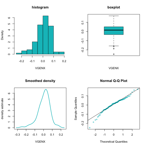

center

The histogram, boxplot and the smoothed density curve show the cc returns are slightly left skewed. The qqplot shows their distribution has fatter tails.

Step 8. Compute all of the relevant descriptive statistics

table.Stats(ret.cc)

##                    VGENX
## Observations    108.0000
## NAs               0.0000
## Minimum          -0.2471
## Quartile 1       -0.0334
## Median            0.0155
## Arithmetic Mean   0.0051
## Geometric Mean    0.0027
## Quartile 3        0.0513
## Maximum           0.1710
## SE Mean           0.0066
## LCL Mean (0.95)  -0.0080
## UCL Mean (0.95)   0.0182
## Variance          0.0047
## Stdev             0.0685
## Skewness         -0.7318
## Kurtosis          1.5469

Indeed, we see the cc returns have a negative skewness and an excess kurtosis of 1.55 compared to the normal distribution.

Step 9. Run the Jarque Bera test to see if the cc returns are normal

jarque.bera.test(ret.cc)

## 
## 	Jarque Bera Test
## 
## data:  ret.cc
## X-squared = 20.407, df = 2, p-value = 3.704e-05

Because the p-value is extremely small, we have strong evidence to reject the null hypothesis that the continously compounded monthly returns for VGENX are normally distributed.

Step 10. Plot autocorrelations over time lags

acf(ret.cc$VGENX)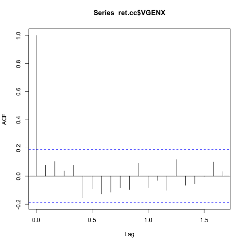

center

The monthly cc returns doesn’t appear to be correlated over time.

Step 11. Compute the annualized continuously compounded mean return and volatility

ret.cc.annual = apply(return_matrix, 2, mean) * 12 
print(ret.cc.annual)

##      VGENX 
## 0.06134274

vol.cc.annual = apply(return_matrix, 2, sd) * sqrt(12)
print(vol.cc.annual)

##     VGENX 
## 0.2372199

Step 12. Compute the annualized simple mean return

exp(ret.cc.annual) - 1

##      VGENX 
## 0.06326327

Categories