Download Stock Price Data Using R

Downloading and charting stock prices data become easy when using the tseries and PerformanceAnalytics R packages.

Step 1. Load these libraries.

library(PerformanceAnalytics)
library(zoo)
library(tseries)

Step 2. Download the monthly adjusted closing price data on S&P500 (^GSPC) and NovaGold (NG) between Jan 2004 and Sept 2014 from Yahoo using the function get.hist.quote() from the tseries package.

sp500 = get.hist.quote(instrument="^GSPC", start="2004-01-01", 
                       end="2014-09-30", origin="1970-01-01",
                       quote="AdjClose", provider="yahoo", 
                       compression="m", retclass="zoo")

## time series starts 2004-01-02
## time series ends   2014-09-02

ng = get.hist.quote(instrument="NG", start="2004-01-01", 
                    end="2014-09-30", origin="1970-01-01",
                    quote="AdjClose", provider="yahoo", 
                    compression="m", retclass="zoo")

## time series starts 2004-01-02
## time series ends   2014-09-02

Step 3. Change the class of the time index to yearmon which is appropriate for monthly data using as.yearmon() in the zoo package.

index(sp500) = as.yearmon(index(sp500))
index(ng) = as.yearmon(index(ng))

# inspect the price data
cat("Start: ", as.character(start(sp500)), "  End: ", as.character(end(sp500)))

## Start:  Jan 2004   End:  Sep 2014

cat("Start: ", as.character(start(ng)), "  End: ", as.character(end(ng)))

## Start:  Jan 2004   End:  Sep 2014

Step 4. Put both SP500 and NG price data in one data frame to make it easier for analysis.

prices = merge(sp500, ng)
colnames(prices) = c("SP500", "NG")

Step 5. Calculate continuously compounded returns as difference in log prices.

ret.cc = diff(log(prices))

# inspect the return data
cat("Start: ", as.character(start(ret.cc)), "  End: ", as.character(end(ret.cc)))

## Start:  Feb 2004   End:  Sep 2014

head(ret.cc, 3)

##                SP500          NG
## Feb 2004  0.01213504 -0.03889948
## Mar 2004 -0.01649420  0.04689952
## Apr 2004 -0.01693331 -0.27842887

Step 6. Plot returns using chart.TimeSeries() and chart.Bar() in the PerformanceAnalytics package.

chart.TimeSeries(ret.cc, legend.loc="bottomright", main="", 
                 ylab="monthly cc return")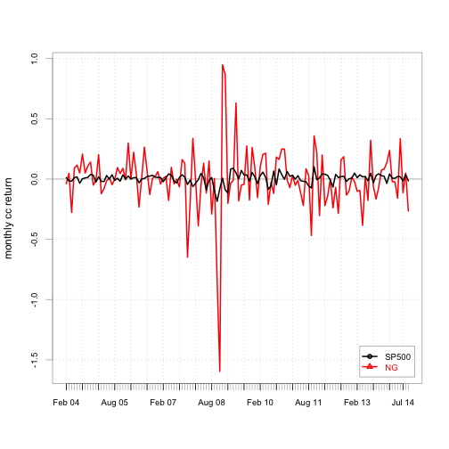

center

chart.Bar(ret.cc, legend.loc="bottomright", main="", 
          ylab="monthly cc return")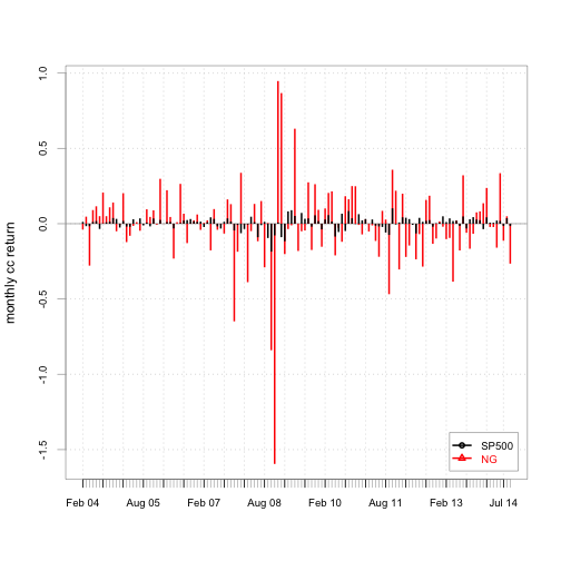

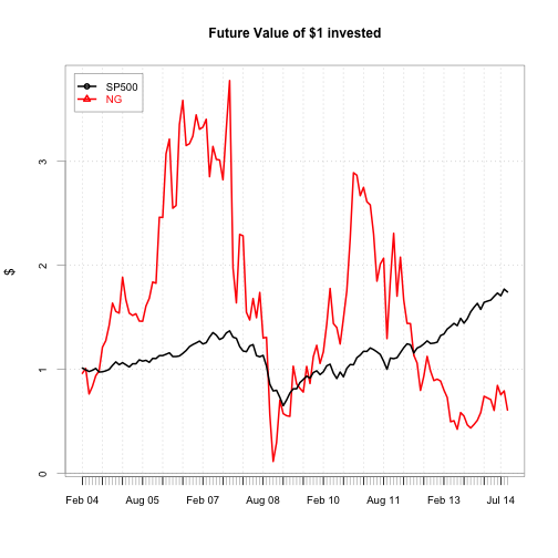
center

Step 7. Plot cumulative returns using chart.CumReturns() in the PerformanceAnalytics package. Note we need to use simple returns instead of continuously compounded returns for this, so we first calcualte the simple returns using diff() and lag() on the price data.

ret.simple = diff(prices) / lag(prices, k=-1)
chart.CumReturns(ret.simple, legend.loc="topleft", wealth.index=TRUE, 
                 ylab="$", main="Future Value of $1 invested")

center

Categories