When predicting numeric values, the root mean squared error (RMSE) is frequently used as a model evaluation measure. The smaller, the better. Its calculation is intuitive:
- take the difference between each actual/observed value and the prediction (its official name is “residual”, meaning leftover after subtracting the predicted values from the actual observed ones),
- square it,
- average over all differences,
- take the square root.
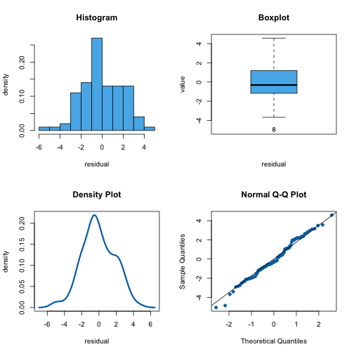
So RMSE measures how far on average the predicted values are from the actual values. In addition to look at RMSE, we can also look at the distribution of all the residuals. The following plots shows a simulated example.
set.seed(92)

y = 1:100
yhat = y + rnorm(100, 0, 2)

dat = data.frame(residual = y - yhat, yhat=yhat)
plt = ezplot::plt_dist(dat)
plt("residual")
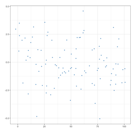
And we can plot the residuals against the predicted values. Its technical term is “residual plot.” The residual plot for the same example is shown below. In this particular example, we see the residuals center around zero randomly and there’s no trend or variation across the predicted values (horizontally).
plt = ezplot::mk_scatterplot(dat)
plt("yhat", "residual")
