This is the first article of a series on how environments work in R. If this
sounds foreign to you, you’re probably wondering, “what is a R environment?”
Don’t. Instead, ask “what does a R environment do?” This is because 99% of the
utility lies in understanding how it behaves. And yes, you can understand how it
behaves without knowing what it is, which is confusing given that different
things are carelessly named the same in the official R manual. For now, just
think of environment as a container. Or if you want, you can even take its
english meaning (after all, programmers try to name things vividly). Every time
you open Rstudio, you’re inside an environment called the global environment.
How do I know that? You can check it yourself by running the following command
inside Rstudio. It tells you the current envionment you’re in.
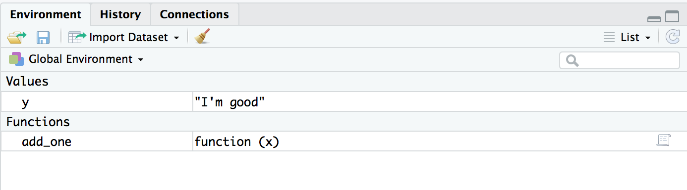
environment()## <environment: R_GlobalEnv>Take a look at the Environment panel and notice the global env is currently empty. Let’s put some stuff inside by running the following code block.
y = "I'm good"
add_one = function(x) {
        y = x + 1
        g = function() y
        g()
}
Look at the Environment panel again and notice the global env now has y and add_one.
What happens if I call add_one(1)? It returns 2. We see the
value of y defined outside of the add_one function doesn’t affect the
value of y defined inside. But what’s really going on under the hood?
The call add_one(1) happened in the global env as I simply ran it inside
Rstudio without changing the current environment. We say the global env is the
calling environment of the function add_one(). If we search for y
inside the function’s calling environment, we’ll get a value of “I’m good.”
Obviously, this was not what R did when we ran add_one(1) because otherwise,
R would’ve returned an error as a result of adding a string and integer. So what
did R do?
When we sent add_one(1) to R (or when add_one(1) was evaluated), a new
environment was created, with x placed inside and associated with the value 1.
Let’s call this new environment \(e_1\).
Next, the expression y = x + 1 was evaluated in \(e_1\), and R searched for
x first in \(e_1\) and found its value to be 1. Addition was carried out and
y was created in \(e_1\) and associated with a value of 2.
Next, the expression g = function() y was evaluated in \(e_1\). As a
result, g was created in \(e_1\) and associated with a function
function() y.
Finally, the expression g() was evaluated in \(e_1\). This created another
new environment with nothing inside. Let’s call it \(e_2\). The body of g
asks to return y, this made R search for y, first inside \(e_2\) and found
nothing, and then inside \(e_1\) and found a value of 2. Under the
hood, R could move to \(e_1\) after done with \(e_2\) because \(e_2\) was
pointed to \(e_1\) by a pointer. We call \(e_1\) is the parent (environment) of
\(e_2\). In general, whenever R cannot find an object inside an environment,
it’ll look for it in its parent environment.
This concludes the first article of the series. If you’re not confused yet, click here for the second article, which provides a high level summary of this first article and shows how the <<- operator works.