Moving Average Models Demo

If you work with time series data, you need to know moving average models. I’m going to show you some basic related R commands.

set.seed(123)

# Simulate 250 observations from the described MA(1) model
ma1_sim = arima.sim(model = list(ma=0.5), n=250, mean=0, sd=0.1) + 0.05
ma2_sim = arima.sim(model = list(ma=0.9), n=250, mean=0, sd=0.1) + 0.05

# Generate the theoretical ACF with upto lag 10
acf_ma1_model = ARMAacf(ma=0.5, lag.max=10)
acf_ma2_model = ARMAacf(ma=0.9, lag.max=10)

# Split plotting window in three rows
par(mfrow=c(3,1))

# First plot: The simulated observations
plot(ma1_sim, type="l", main="MA(1) Process: mu=0.05",
     xlab="time", ylab="y(t)", col="blue")
lines(ma2_sim, type="l", col="red")
abline(h=0)

# Second plot: Theoretical ACF
plot(1:10, acf_ma1_model[2:11], type="h", col="blue", ylab="ACF", 
     main="theoretical ACF")

# Third plot: Sample ACF
tmp = acf(ma1_sim, lag.max=10) # Assign to tmp the Sample ACF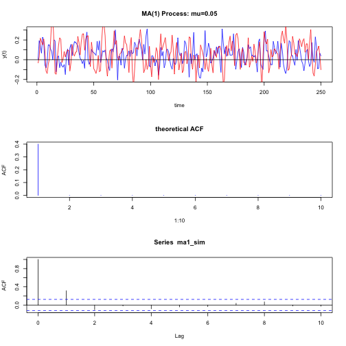

center

str(tmp)

## List of 6
##  $ acf   : num [1:11, 1, 1] 1 0.3133 -0.1035 -0.0206 -0.0818 ...
##  $ type  : chr "correlation"
##  $ n.used: int 250
##  $ lag   : num [1:11, 1, 1] 0 1 2 3 4 5 6 7 8 9 ...
##  $ series: chr "ma1_sim"
##  $ snames: NULL
##  - attr(*, "class")= chr "acf"

# Reset graphical window to only one graph
par(mfrow=c(1,1))

Categories